Image Handling
Last updated on 2024-10-18 | Edit this page
Estimated time: 120 minutes
Download Chapter notebook (ipynb)
Mandatory Lesson Feedback Survey
Overview
Questions
- How to read and process images in Python?
- How is an image mask created?
- What are colour channels in images?
- How do you deal with big images?
Objectives
- Understanding 2-dimensional greyscale images
- Learning image masking
- 2-dimensional colour images and colour channels
- Decreasing memory load when dealing with images
Prerequisites
- NumPy arrays
- Plots and subplots with matplotlib
Practice Exercises
This lesson has no explicit practice exercises. At each step, use images of your own choice to practice. There are many image file formats, different colour schemes etc for which you can try to find similar or analogous solutions.
Challenge
Reading and Processing Images
In biology, we often deal with images; for example, microscopy and different medical imaging modalities often output images and image data for analysis. In many cases, we wish to extract some quantitative information from these images. The focus of this lesson is to read and process images in Python. This will include:
- Working with 2-dimensional greyscale images
- Creating and applying binary image masks
- Working with 2-dimensional colour images, and interpreting colour channels
- Decreasing the memory for further processing by reducing resolution or patching
- Working with 3-dimensional images
Image Example
The example in Figure 1 is an image from the cell image library with the following description:
“Midsaggital section of rat cerebellum, captured using confocal imaging. Section shows inositol trisphosphate receptor (IP3R) labelled in green, DNA in blue, and synaptophysin in magenta. Honorable Mention, 2010 Olympus BioScapes Digital Imaging Competition®.”
Given this information, we might want to determine the relative amounts of IP3R, DNA and synaptophysin in this image. This tutorial will guide you through some of the steps to get you started with processing images of all types, using Python. You can then refer back to this image analysis example, and perform some analyses of your own.

Work-Through Example
Reading and Plotting a 2-dimensional Image
Firstly, we must read an image in. To demonstrate this we can use the
example of a histological slice through an axon bundle. We use
Matplotlib’s image module, from which we import the function
imread, used to store the image in a variable that we will
name img. The function imread can interpret
many different image formats, including .jpg, .png and .tif images.
OUTPUT
PIL.UnidentifiedImageError: cannot identify image file 'fig/axon_slice.jpg'We can then check what type of variable is, using the type() function:
OUTPUT
NameError: name 'img' is not definedThis tells us that the image is stored in a NumPy array;
ndarray here refers to an N-dimensional array. We can check
some other properties of this array, for example, what the image
dimensions are, using the .shape attribute:
OUTPUT
NameError: name 'img' is not defined
This tells us that our image is composed of 2300 by 3040 data units, or
pixels as we are dealing with an image. The total number of
pixels in the image, is equivalent to its resolution. In digital
imaging, a pixel is simply a numerical value that represents either
intensity, in a greyscale image; or colour in a colour image. Therefore,
as data, a two-dimensional (2-D) greyscale image comprises a 2-D array
of these intensity values, or elements; hence the name ‘pixel’ is an
amalgamation of ‘picture’ and ‘element’. The array in our example has
two dimensions, and so we can expect the image to be 2-D as well. Let us
now use matplotlib.pyplot’s imshow function to plot the
image to see what it looks like. We can set the colour map to
gray in order to overwrite the default colour map.
PYTHON
from matplotlib.pyplot import subplots, show

fig, ax = subplots(figsize=(25, 15))

ax.imshow(img, cmap='gray');
imshow has allowed us to plot the NumPy array of our image
data as a picture. The figure is divided up into a number of pixels, and
each of these is assigned an intensity value, which is held in the NumPy
array. Let’s have a closer look by selecting a smaller region of our
image and plotting that.
PYTHON
from matplotlib.pyplot import subplots, show

fig, ax = subplots(figsize=(25, 15))

ax.imshow(img[:50, :70], cmap='gray');
OUTPUT
NameError: name 'img' is not defined
By using img[:50, :70] we can select the first 50 values
from the first dimension, and the first 70 values from the second
dimension. Note that using a colon denotes ‘all’, where ‘:50’ is
inclusive of every number up to 50, for example. Thus, the image above
shows a very small part of the upper left corner of our original image.
As we are now zoomed in quite close to that corner, we can easily see
the individual pixels here.
OUTPUT
NameError: name 'img' is not defined
We have now displayed an even smaller section from that same upper left
corner of the image. Each square is a pixel and it has a single grey
value. Thus, the pixel intensity values are assigned by the numbers
stored in the NumPy array, img. Let us have a look at these
values by producing a slice from the array.
OUTPUT
NameError: name 'img' is not definedEach of these numbers corresponds to an intensity in the specified colourmap. These numbers range from 0 to 255, implying 256 shades of grey.
We chose cmap = gray, which assigns darker grey colours to
smaller numbers, and lighter grey colours to higher numbers. However, we
can also pick a non-greyscale colour map to plot the same image. We can
even display a colourbar to keep track of the intensity values.
Matplotlib has a diverse palette of colour maps that you can look
through, linked here.
Let’s take a look at two commonly-used Matplotlib colour maps called
viridis and magma:
PYTHON
fig, ax = subplots(nrows=1, ncols=2, figsize=(25, 15))

p1 = ax[0].imshow(img[:20, :15], cmap='viridis')
p2 = ax[1].imshow(img[:20, :15], cmap='magma')
fig.colorbar(p1, ax=ax[0], shrink = 0.8)
fig.colorbar(p2, ax=ax[1], shrink = 0.8);

show()
Note, that even though we can plot our greyscale image with colourful
colour schemes, it still does not qualify as a colour image. These are
just false-colour, Matplotlib-overlayed interpretations of rudimentary
intensity values. The reason for this is that a pixel in a standard
colour image actually comprises three sets of
intensities per pixel; not just the one, as in this greyscale example.
In the case above, the number in the array represented a grey value and
the colour was assigned to that grey value by Matplotlib.
These represent ‘false’ colours.
Creating an Image Mask
Now that we know that images essentially comprise arrays of numerical intensities held in a NumPy array, we can start processing images using these numbers.
As an initial approach, we can plot a histogram of the intensity values
that comprise an image. We can make use of the .flatten()
method to turn the original 2300 x 3040 array into a one-dimensional
array with 6,992,000 values. This rearrangement allows the numbers
within the image to be represented by a single column inside a matrix or
DataFrame.
The histogram plot shows how several instances of each intensity make up this image:
PYTHON
fig, ax = subplots(figsize=(10, 4))

ax.hist(img.flatten(), bins = 50)
ax.set_xlabel("Pixel intensity", fontsize=16);

show()
The image displays a slice through an axon bundle. For the sake of example, let’s say that we are now interested in the myelin sheath surrounding the axons (the dark rings). We can create a mask that isolates pixels whose intensity value is below a certain threshold (because darker pixels have lower intensity values). Everything below this threshold can be assigned to, for instance, a value of 1 (representing True), and everything above will be assigned a value of 0 (representing False). This is called a binary or Boolean mask.
Based on the histogram above, we might want to try adjusting that threshold somewhere between 100 and 200. Let’s see what we get with a threshold set to 125. Firstly, we must implement a conditional statement in order to create the mask. It is then possible to apply this mask to the image. The result can be that we plot both the mask and the masked image.
PYTHON
threshold = 125

mask = img < threshold

img_masked = img*mask

fig, ax = subplots(nrows=1, ncols=2, figsize=(20, 10))

ax[0].imshow(mask, cmap='gray')
ax[0].set_title('Binary mask', fontsize=16)
ax[1].imshow(img_masked, cmap='gray')
ax[1].set_title('Masked image', fontsize=16)

show()
The left subplot shows the binary mask itself. White represents values where our condition is true, and black where our condition is false. The right image shows the original image after we have applied the binary mask, it shows the original pixel intensities in regions where the mask value is true.
Note that applying the mask means that the intensities where the condition is true are left unchanged. The intensities where the condition is false are multiplied by zero, and therefore set to zero.
Let’s have a look at the resulting image histograms.
PYTHON
fig, ax = subplots(nrows=1, ncols=2, figsize=(20, 5))

ax[0].hist(img_masked.flatten(), bins=50)
ax[0].set_title('Histogram of masked image', fontsize=16)
ax[0].set_xlabel("Pixel intensity", fontsize=16)

ax[1].hist(img_masked[img_masked != 0].flatten(), bins=25)
ax[1].set_title('Histogram of masked image after zeros are removed', fontsize=16)
ax[1].set_xlabel("Pixel intensity", fontsize=16)

show()
The left subplot displays the values for the masked image. Note that there is a large peak at zero, as a large part of the image is masked. The right subplot histogram, however, displays only the non-zero pixel intensities. From this, we can see that our mask has worked as expected, where only values up to 125 are found. This is because our threshold causes a sharp cut-off at a pixel intensity of 125.
Colour Images
So far, our image has had a single intensity value for each pixel. In colour images, we have multiple channels of information per pixel; most commonly, colour images are RGB, comprising three corresponding to intensities of red, green and blue. There are many other formats of colour image, but these will be beyond the scope of this lesson. In a RGB colour image, any colour will be a composite of the intensity value for each of these colours. Our chosen example for a colour image is one of the rat cerebellar cortex. Let us firstly import it and check its shape.
OUTPUT
PIL.UnidentifiedImageError: cannot identify image file 'fig/rat_brain_low_res.jpg'OUTPUT
NameError: name 'img_col' is not definedOur image array now contains three dimensions: the first two are the spatial dimensions corresponding to the pixel positions as x-y coordinates. The third dimension contains the three colour channels, corresponding to three layers of intensity values (red, blue and green) on top of each other, per pixel. First, let us plot the entire image using Matplotlib’s imshow method.
First, let us plot the whole image.
OUTPUT
NameError: name 'img_col' is not defined
We can then visualise the three colour channels individually by slicing the NumPy array comprising our image. The stack with index 0 corresponds to ‘red’, index 1 corresponds to ‘green’ and index 2 corresponds to ‘blue’:
OUTPUT
NameError: name 'img_col' is not definedOUTPUT
NameError: name 'img_col' is not definedOUTPUT
NameError: name 'img_col' is not definedPYTHON
fig, ax = subplots(nrows=1, ncols=3, figsize=(20, 10))

imgplot_red = ax[0].imshow(red_channel, cmap="Reds")
imgplot_green = ax[1].imshow(green_channel, cmap="Greens")
imgplot_blue = ax[2].imshow(blue_channel, cmap="Blues")

fig.colorbar(imgplot_red, ax=ax[0], shrink=0.4)
fig.colorbar(imgplot_green, ax=ax[1], shrink=0.4)
fig.colorbar(imgplot_blue, ax=ax[2], shrink=0.4);

show()
This shows what colour combinations each of the pixels is made up of. Notice that the intensities go up to 255. This is because RGB (red, green and blue) colours are defined within an intensity range of 0-255. This gives a vast total 16,777,216 possible colour combinations.
We can plot histograms of each of the colour channels.
PYTHON
fig, ax = subplots(nrows=1, ncols=3, figsize=(20, 5))

ax[0].hist(red_channel.flatten(), bins=50)
ax[0].set_xlabel("Pixel intensity", fontsize=16)
ax[0].set_xlabel("Red channel")
ax[1].hist(green_channel.flatten(), bins=50)
ax[1].set_xlabel("Pixel intensity", fontsize=16)
ax[1].set_xlabel("Green channel")
ax[2].hist(blue_channel.flatten(), bins=50)
ax[2].set_xlabel("Pixel intensity", fontsize=16)
ax[2].set_xlabel("Blue channel")

show()
Dealing with Large Images
Often, we encounter situations where we have to deal with very large images that are composed of many pixels. Images such as these are often difficult to process, as they can require a lot of computer memory when they are processed. We will explore two different strategies for dealing with this problem - decreasing resolution, and using patches from the original image. To demonstrate this, we can make use of the full-resolution version of the rat brain image in the previous example.
OUTPUT
PIL.UnidentifiedImageError: cannot identify image file 'fig/rat_brain.jpg'
NameError: name 'img_hr' is not defined
When attempting to read the image in using the imread() function, we receive a warning from python indicating that the “Image size (324649360 pixels) exceeds limit of 178956970 pixels, could be decompression bomb DOS attack.” This is alluding to a potential malicious file, designed to crash or cause disruption by using up a lot of memory.
We can get around this by changing the maximum pixel limit, as follows.
To do this, we will need to the Image module from the Python Image Library (PIL), as follows:
Let’s try again. Please be patient, as this might take a moment.
OUTPUT
PIL.UnidentifiedImageError: cannot identify image file 'fig/rat_brain.jpg'OUTPUT
NameError: name 'img_hr' is not definedNow we can plot the full high-resolution image:
OUTPUT
NameError: name 'img_hr' is not defined
Although now we can plot this image, it does still consist of over 300 million pixels, which could run us into memory problems when attempting to process it. One approach is simply to reduce the resolution by importing the image using the Image module from the PIL library: which we imported in the code given, above. This library gives us a wealth of tools to process images, including methods to decrease an image’s resolution. PIL is a very rich library with a multitude of useful tools. As always, having a look at the official documentation and playing around with it yourself is highly encouraged.
We can make use of the resize method to downsample the
image, providing the desired width and height as numerical arguments, as
follows:
PYTHON
img_pil = Image.open('fig/rat_brain.jpg')
img_small = img_pil.resize((174, 187))

print(type(img_small))
OUTPUT
PIL.UnidentifiedImageError: cannot identify image file 'fig/rat_brain.jpg'
NameError: name 'img_pil' is not defined
NameError: name 'img_small' is not defined
Plotting should now be considerably quicker.
OUTPUT
NameError: name 'img_small' is not defined
Using the above code, we have successfully resized the image to a
resolution of 174 x 187 pixels. It is, however, important to note that
our image is no longer in the format of a NumPy array, but rather it now
has the type PIL.Image.Image. We can, however, easily
convert it back into a NumPy array using the array function, if we so
wish.
OUTPUT
NameError: name 'img_small' is not definedOUTPUT
NameError: name 'img_numpy' is not definedDespite the above, it is often desired to keep images in their full resolution, as resizing effectively results in a loss of information. An commonly used, alternative approach to such downsampling is to patch the images. Patching an image essentially divides the picture up into smaller chunks that are termed patches.
For this, we can implement functionality from the Scikit-Learn machine learning library.
The extract_patches_2d function is used to extract parts
of the image. The shape of each patch, together with the maximal number
of patches, can be specified, as follows:
OUTPUT
NameError: name 'img_hr' is not definedOUTPUT
NameError: name 'patches' is not defined
When using the .shape attribute, the output given here
shows that the image has been successfully subdivided into 100 patches,
with resolution 174 x 187 pixels, across three channels: red, blue and
green (as this is an RGB, colour image). Note that patching itself can
be a memory-intensive task. Extracting lots and lots of patches may take
a long time. To look at the patches, we can make use of a for loop to
iterate through the first element of the .shape array (the
100 patches), and visualise each one on its own subplot using the
.imshow method, as follows:
PYTHON
fig, ax = subplots(nrows=10, ncols=10, figsize=(25, 25))

ax = ax.flatten()

for index in range(patches.shape[0]):
    ax[index].imshow(patches[index, :, :, :])
OUTPUT
NameError: name 'patches' is not defined
Working with these smaller, individual patches will be much more manageable and computationally resourceful.
3D Images
So far, we have covered how to handle two-dimensional image data in a variety of ways. But scenarios will often arise whereby the analysis of three-dimensional image data is required. A good example of such 3-D images that is commonly encountered, is MRI scans. These don’t natively exist as .csv format, but are often delivered in specialised image formats. One such format is nii: the Neuroimaging Informatics Technology Initiative (NIfTI) open file format. Handling these types of images requires specialised software. In particular, we will be using an open-source library called nibabel. Documentation for this package is available at https://nipy.org/nibabel/.
As it is not contained in your Python installation by default, it needs to be installed first.
Two methods for installing this, are given here. If you have previously installed the Anaconda distribution of Python, paste the following onto your command line or terminal, and hit return:
conda install -c conda-forge nibabelAlternatively, you can also install it using Python’s default package installer ‘pip’ by pasting the following onto your command line or terminal, and hitting return:
pip install nibabelin your command line or terminal.
The package is now available for use. To shorten how we call on the
nibabel package in our code, we can use the above import statement,
using the alias nib to refer to nibabel. Thus we can call
on any function in nibabel, by using nib is followed by a
period and the name of that specific function, as follows:
OUTPUT
<class 'numpy.memmap'>OUTPUT
(256, 256, 124)We can see that the .shape attribute revelas that this image has three dimensions, and a total of 256 x 256 x 124 volume pixels (or voxels). To visualise our image, we can plot one slice at a time. The example below shows three different slices, in the transverse direction (from chin to the top of the head). To access an image across the transverse orientation, a single value is selected from the third dimension of the image, as follows. As always, the colons indicate that all data on the remaining two axes is selected and visualised:
PYTHON
fig, ax = subplots(ncols=3, figsize=(25, 15))

p1 = ax[0].imshow(img_data[:, :, 60], cmap='gray')
p2 = ax[1].imshow(img_data[:, :, 75], cmap='gray')
p3 = ax[2].imshow(img_data[:, :, 90], cmap='gray')

fig.colorbar(p1, ax=ax[0], shrink=0.4)
fig.colorbar(p2, ax=ax[1], shrink=0.4)
fig.colorbar(p3, ax=ax[2], shrink=0.4);

show()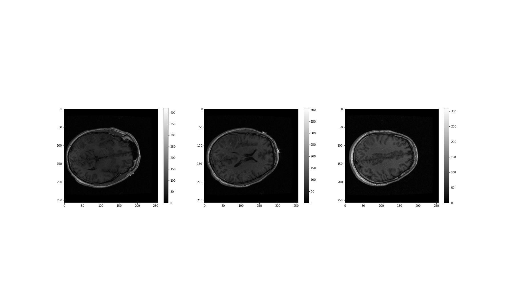
These look fairly dark. We can improve the contrast, by adjusting the
intensity range. This requires intentionally overriding the default
values, and specifying our own for the keyword arguments
vmin and vmax.
The vmin and vmax parameters in matplotlib
define the data range that the colormap (in our case the
grey map) covers; thus they control the range of data
values indicated by the colormap in use. By default, the colormap covers
the complete value range of the supplied data. For instance, in many
images this will typically be somewhere between 0 and 255. If we want to
brighten up the darker shades of grey in our example MRI slices, for
example, we can reduce the value of the vmax parameter.
Expanding upon the above code:
PYTHON
fig, ax = subplots(ncols=3, figsize=(25, 15))

p1 = ax[0].imshow(img_data[:, :, 60], cmap='gray', vmin=0, vmax=150)
p2 = ax[1].imshow(img_data[:, :, 75], cmap='gray', vmin=0, vmax=150)
p3 = ax[2].imshow(img_data[:, :, 90], cmap='gray', vmin=0, vmax=150)

fig.colorbar(p1, ax=ax[0], shrink=0.4)
fig.colorbar(p2, ax=ax[1], shrink=0.4)
fig.colorbar(p3, ax=ax[2], shrink=0.4);

show()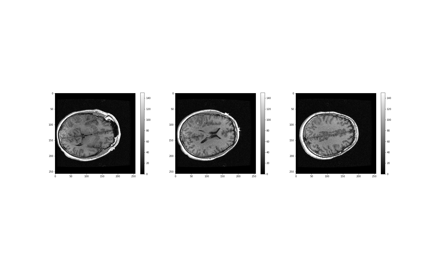
What about the other dimensions? We can also plot coronal and sagittal slices, for example. But take note that, in this case, the respective slices have different pixel resolutions. Let us expand our code even further, to display all three desired viewing planes in our MRI scan, as follows:
PYTHON
fig, ax = subplots(nrows=3, ncols=5, figsize=(26, 18))

t1 = ax[0, 0].imshow(img_data[:, :, 45].T, cmap='gray', vmin=0, vmax=150, origin='lower')
t2 = ax[0, 1].imshow(img_data[:, :, 60].T, cmap='gray', vmin=0, vmax=150, origin='lower')
t3 = ax[0, 2].imshow(img_data[:, :, 75].T, cmap='gray', vmin=0, vmax=150, origin='lower')
t4 = ax[0, 3].imshow(img_data[:, :, 90].T, cmap='gray', vmin=0, vmax=150, origin='lower')
t5 = ax[0, 4].imshow(img_data[:, :, 105].T, cmap='gray', vmin=0, vmax=150, origin='lower')

c1 = ax[1, 0].imshow(img_data[:, 50, :].T, cmap='gray', vmin=0, vmax=150, origin='lower')
c2 = ax[1, 1].imshow(img_data[:, 75, :].T, cmap='gray', vmin=0, vmax=150, origin='lower')
c3 = ax[1, 2].imshow(img_data[:, 90, :].T, cmap='gray', vmin=0, vmax=150, origin='lower')
c4 = ax[1, 3].imshow(img_data[:, 105, :].T, cmap='gray', vmin=0, vmax=150, origin='lower')
c5 = ax[1, 4].imshow(img_data[:, 120, :].T, cmap='gray', vmin=0, vmax=150, origin='lower')

s1 = ax[2, 0].imshow(img_data[75, :, :].T, cmap='gray', vmin=0, vmax=150, origin='lower')
s2 = ax[2, 1].imshow(img_data[90, :, :].T, cmap='gray', vmin=0, vmax=150, origin='lower')
s3 = ax[2, 2].imshow(img_data[105, :, :].T, cmap='gray', vmin=0, vmax=150, origin='lower')
s4 = ax[2, 3].imshow(img_data[120, :, :].T, cmap='gray', vmin=0, vmax=150, origin='lower')
s5 = ax[2, 4].imshow(img_data[135, :, :].T, cmap='gray', vmin=0, vmax=150, origin='lower');

show()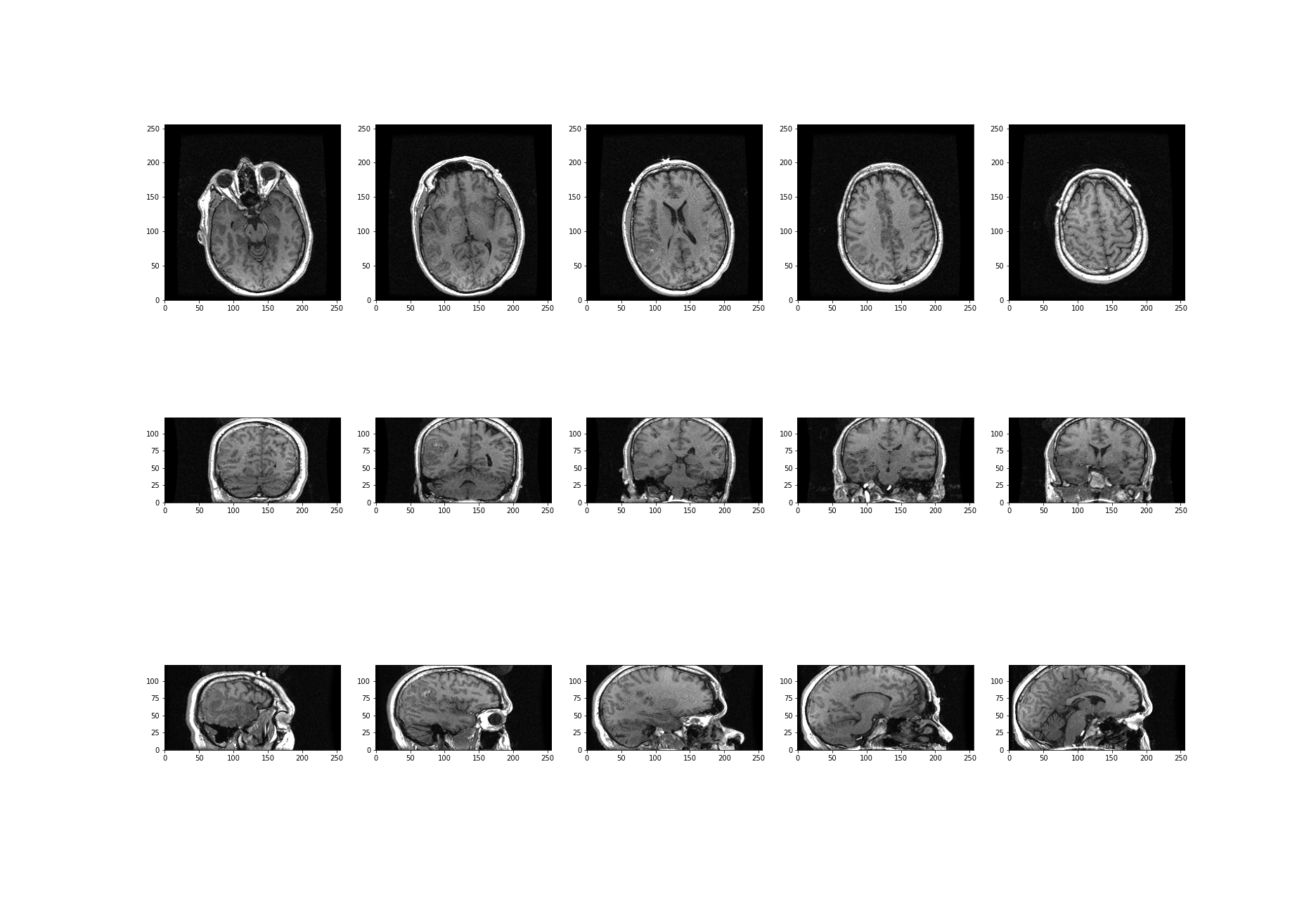
The result is that we have clearly visualised slices of our 3-D image, representing all three viewing planes in this 3-dimensional brain scan.
Exercises
End of chapter Exercises
Assignment
Using the image from the beginning of this lesson (rat_cerebellum.jpg) to perform the following tasks:
Import the image and display it.
Show histograms for each of the colour channels and plot the contributions of each of the RGB colours to the final image, separately.
Create three different binary masks using manually determined thresholds: one for mostly red pixels, one for mostly green pixels, and one for mostly blue pixels. Note that you can apply conditions that are either greater or smaller than a threshold of your choice.
Plot the three masks and the corresponding masked images.
Using your masks, approximate the relative amounts of synaptophysin, IP3R, and DNA in the image. To do this, you can assume that the number of red pixels represents synaptophysin, green pixels represents IP3R and blue pixels represent DNA. The results will vary depending on the setting of the thresholds. How do different threshold values change your results?
Change the resolution of your image to different values. How does the resolution affect your results?
Key Points
- The
imreadfunction can be used to read in and interpret multiple image formats. - Masking isolates pixels whose intensity value is below a certain threshold.
- Colour images typically comprise three channels (corresponding to red, green and blue intensities).
- Python Image Library (PIL) helps to set and raise default pixel limits for reading in and handling larger images.