Getting started
Variables, Types, and Operations
Figure 1
Figure 2
Figure 3
Figure 4
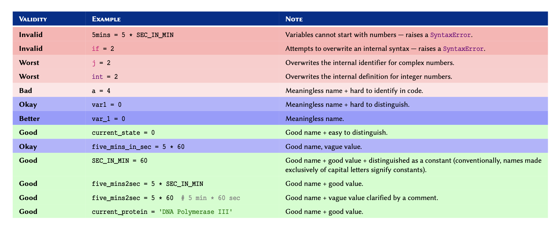
Figure 5
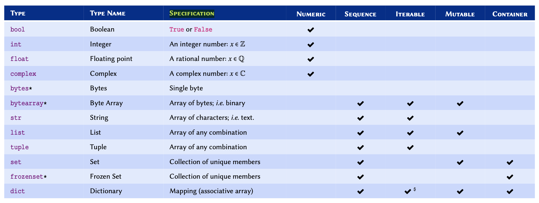 A comprehensive (but non-exhaustive) reference of built-in (native)
types in Python 3.
* Not discussed in this course —
included for reference only.
$dict is not
an iterable by default, however, it is possible to iterate through its
keys.
Figure 6
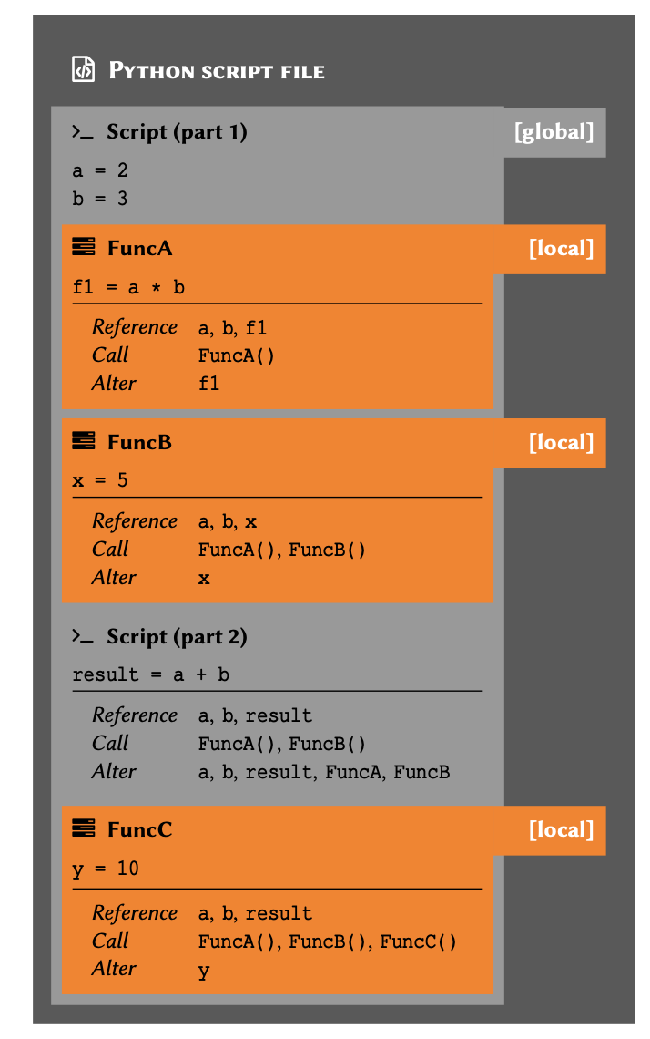
Figure 7
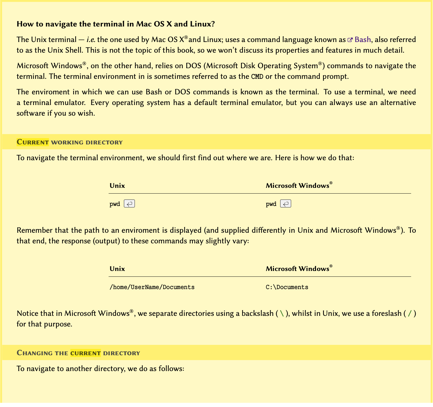

Figure 8
Figure 9
Figure 10
Figure 11

Figure 12

Figure 13

Conditional Statements
Figure 1
Figure 2
In previous chapter, Practice Exercise
11, we explored the implication of CAG repeats in
Huntington’s disease. We also created a polynucleotide chain containing
36 repetition of the CAG codons.
Write a conditional statement that tests the length of a polyQ tract to determine the classification and the disease status based on the following Table:
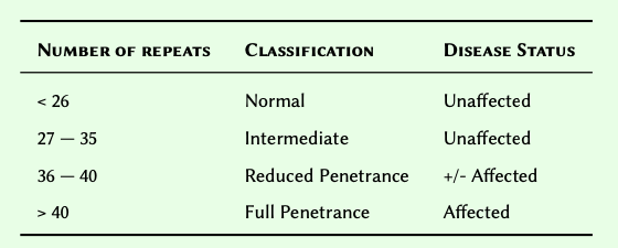
Using the technique you used in Practice Exercise 11, create 5 polyQ tracts containing 26, 15, 39, 32, 36, and 54 codons. Use these polynucleotide chains to test your conditional statement.
Display the result for each chain in the following format:
PolyQ chain with XXX number of CAG codons:
Status: XXX
Classification: XXX
Hint: The length of a polyQ tract represents the number
of nucleotides, not the number of CAG codons. See task 4 of
Practice Exercise
11 for additional information.
Introduction to Arrays
Figure 1
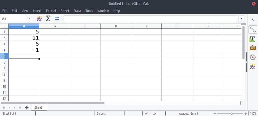
Figure 2
Indexing
In an array, an index is an integer (whole number) that corresponds to a specific item in that array.
You can think of an index as a unique reference or key that corresponds to a specific row in a table. We don’t always write the row number when we create a table. However, we always know that the third row of a table refers to us starting from the first row (row #1), counting three rows down and there we find the third row.
Python, however, uses what we term zero-based indexing. We don’t count the first row as row #1; instead, we consider it to be row #0. As a consequence of starting from #0, we count rows in our table down to row #2 instead of #3 to find the third row. So our table may,essentially, be visualised as follows:
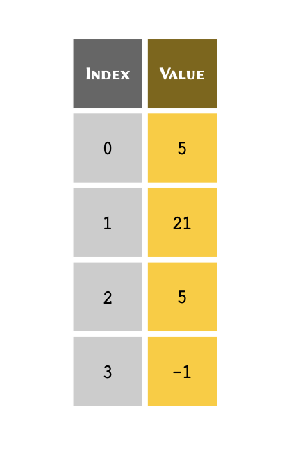
Remember
Python uses zero-based indexing system. This means that the first row of an array, regardless of its type, is always referred to with index #0.
With that in mind, we can use the index for each item in the list, in
order to retrieve it from a list.
Given the following list of four members stored in a
variable called table:
table = [5, 21, 5, -1]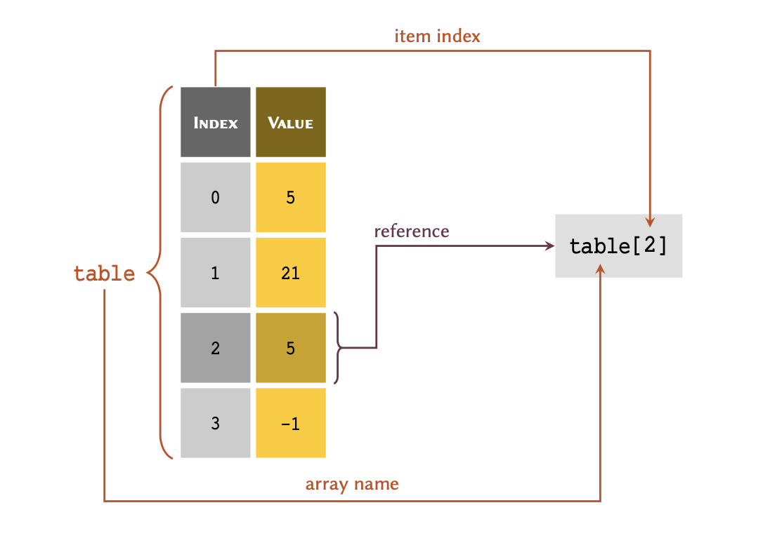
As illustrated in this figure; in order to retrieve a member of an array through its index, we write the name of the variable immediately followed by the index value inside a pair of square brackets — e.g. table[2]. Note, you may have noticed our interchangeable use of the terms ‘list’ and ‘array’. That is because a list, in Python, can be considered as a type of dynamic array (they can increase or decrease in size, as required).
OUTPUT
5OUTPUT
5OUTPUT
-1Practice Exercise 2
Retrieve and display the 5th Fibonacci number from the
list you created in the previous Practice Exercise 1.
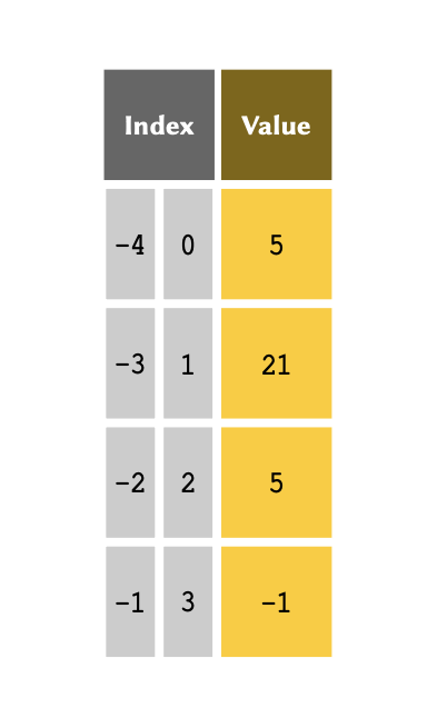
It is sometimes more convenient to index an array, backwards — that is, to reference the members from the bottom of the array, first. This is termed negative indexing, and is particularly useful when we are dealing with lengthy arrays. The indexing system in Python support both positive and negative indexing systems.
The table above therefore may also be represented, as follows:
Remember
Unlike the normal indexing system, which starts from #0, negative indexes start from #-1. This serves to definitely highlight which indexing system is being used.
If the index is a negative number, the indices are counted from the
end of the list. We can implement negative indices in the
same way as positive indices:
OUTPUT
-1OUTPUT
5OUTPUT
21We know that in table, index #-3 refers the same value as index #1. So let us go ahead and test this:
OUTPUT
TrueIf the index requested is larger than the length of the
list minus one, an IndexError will be
raised:
OUTPUT
IndexError: list index out of rangeRemember
The values stored in a list may be referred to as the
members of that list.
Practice Exercise 3
Retrieve and display the last Fibonacci number from the
list you created in Practice Exercise 1.
Figure 3

Figure 4

Figure 5
Figure 6
Figure 7
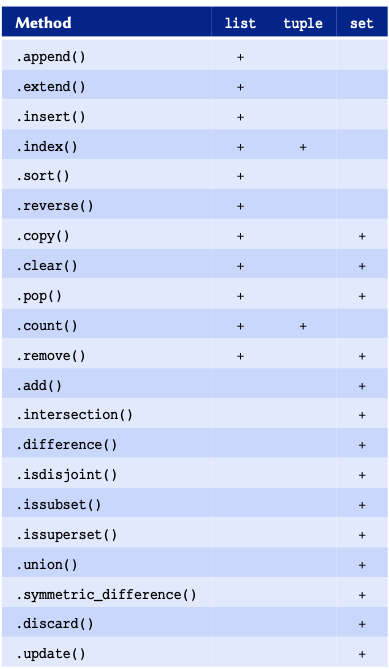
Figure 8
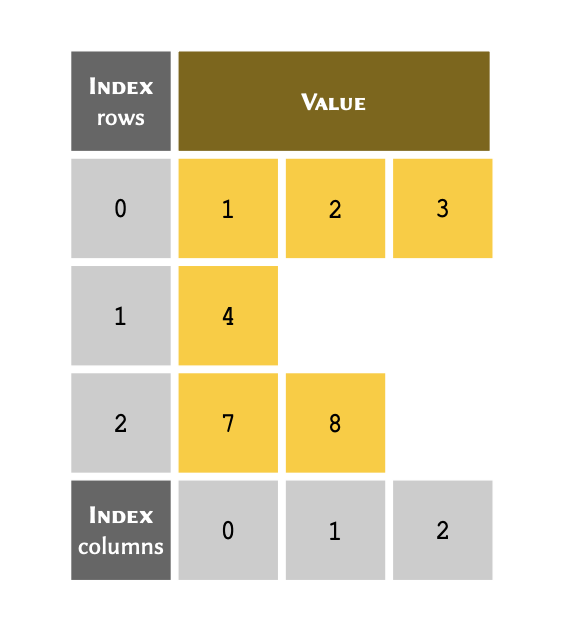
Figure 9
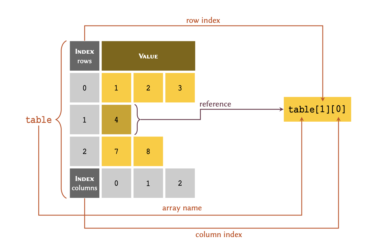
Figure 10
Given the following Table of pathogens and their corresponding diseases:

- Substitute N/A for
None, and create an array to represent the table in its presented order. Retain the array in a variable, and display the result.
- Modify the array you created so that its members are sorted descendingly, and display the result.
Figure 11
A two dimensional arrays may be visualised as follows: 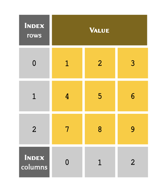
Figure 12
Computers see images as multidimensional arrays (matrices). In its simplest form, an image is a two-dimensional array containing only two colours.
Given the following black and white image:
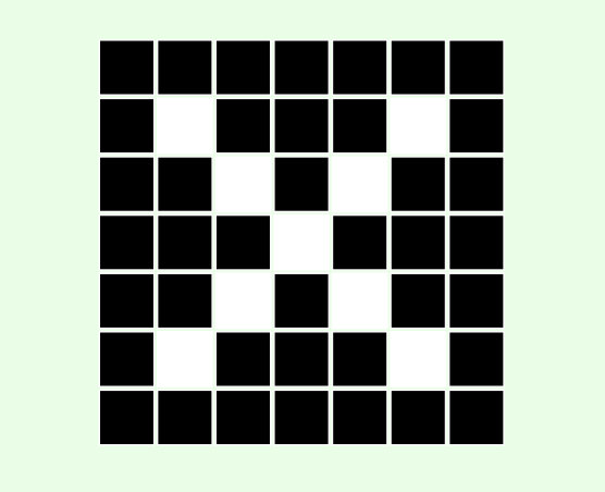
- Considering that black and white squares represent zeros and ones respectively, create a two-dimensional array to represent the image. Display the results.
- Create a new array, but this time use
FalseandTrueto represent black and white respectively.
Display the results.
Figure 13
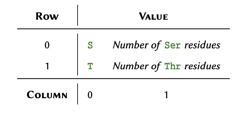
Figure 14
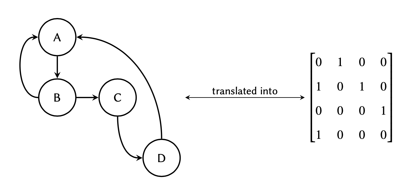 where each row in the matrix
represents a node of origin in the graph, and each column a node of
destination:
Figure 15
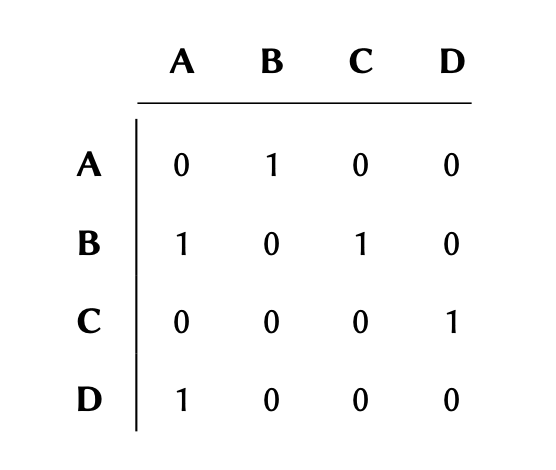 If the graph maintains a
connection (edge) between two nodes (e.g. between nodes A and B in the graph above), the
corresponding value between those nodes would be #1 in the matrix, and
if there are no connections, the corresponding value would #0.
Figure 16
Given the following graph: 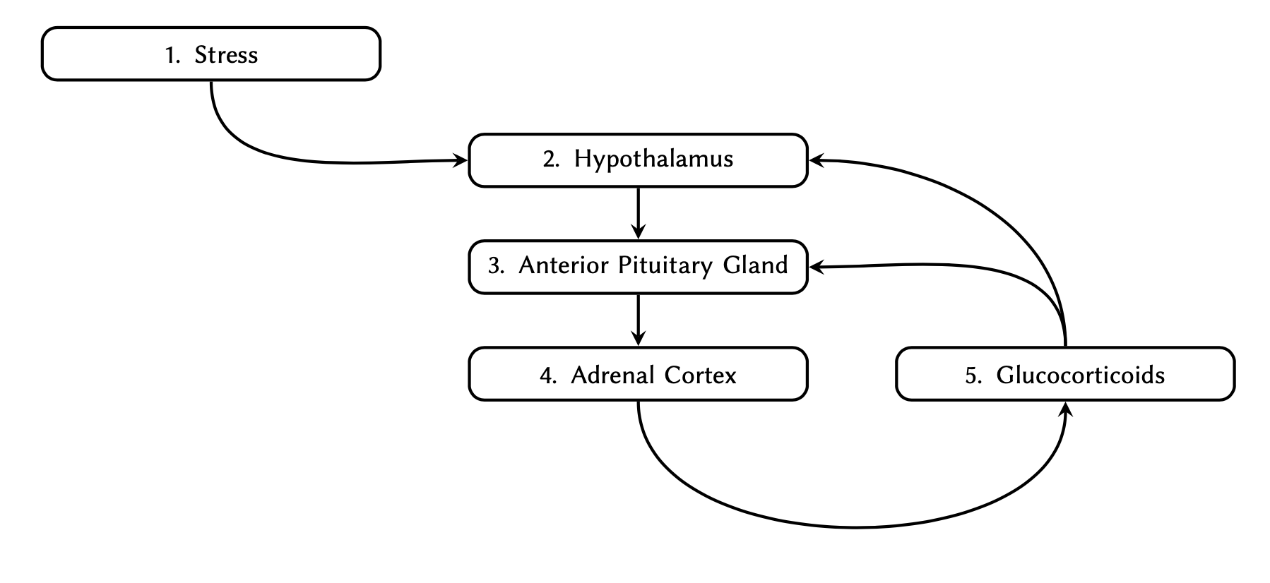
Iterations
Figure 1
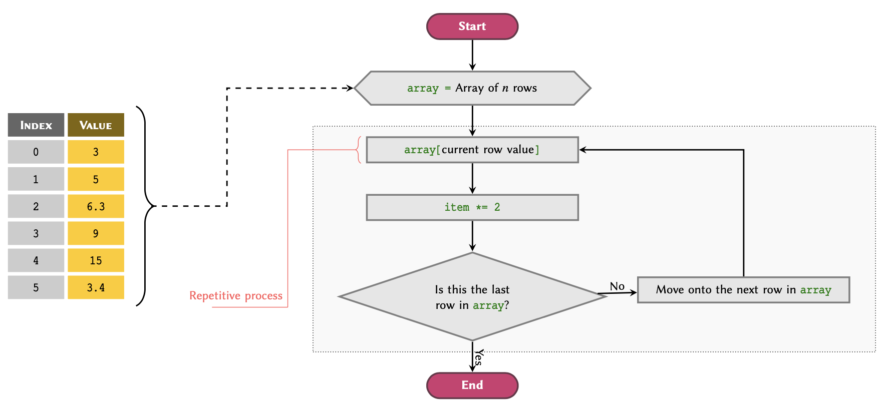
for–loop workflow
applied to a list array.Figure 2
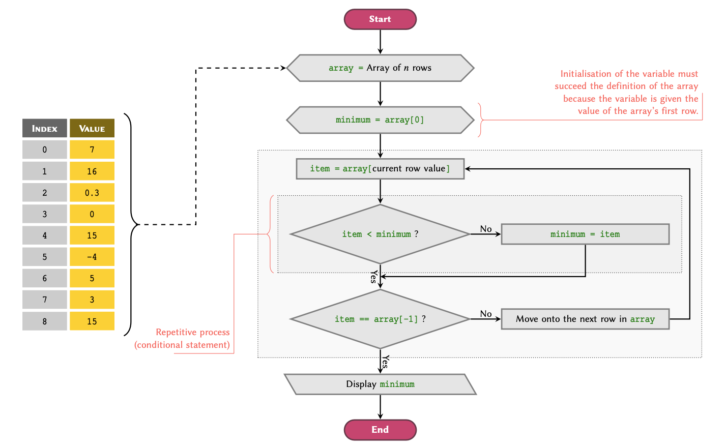
Figure 3
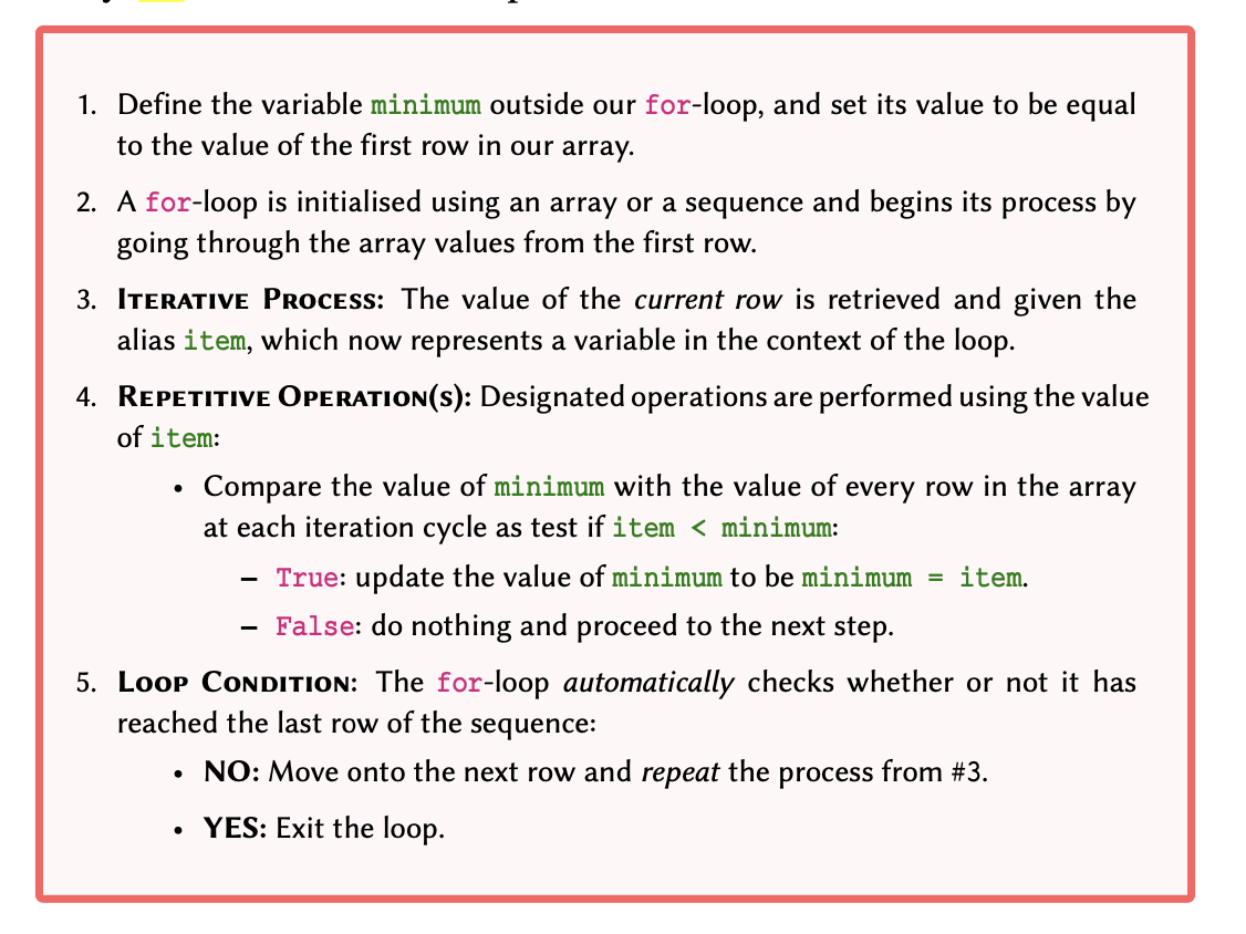
Figure 4

Figure 5
Figure 6
Dictionaries
Figure 1
 One way to associate the proteins with their definitions would be to
make use of nested arrays, as covered in Basic Python 2. However, this
would make it difficult to retrieve the values at a later point in time.
This is because in order to retrieve these values, we would need to know
the numerical index at which a given protein is stored, and the level
it’s stored at.
Figure 2
Functions
Figure 1
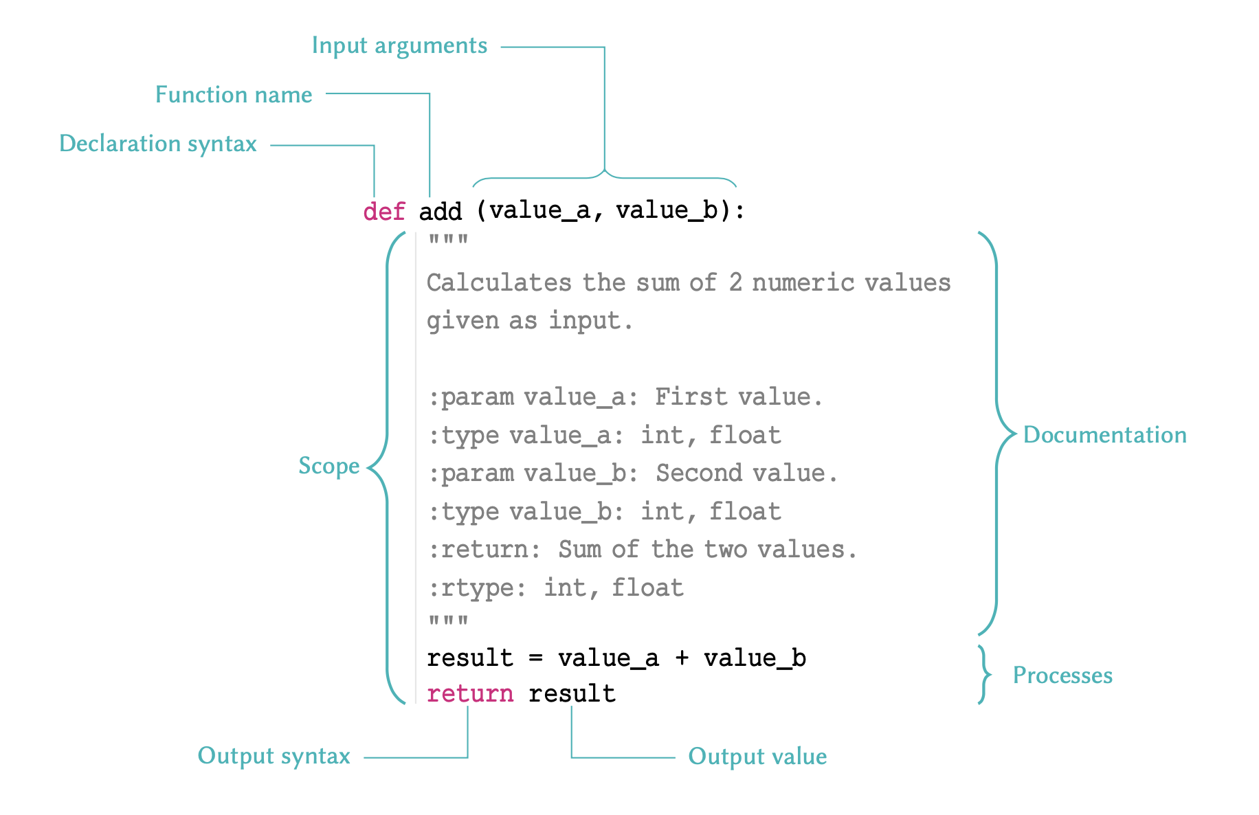
Figure 2
